Welcome

Welcome to Workshop 6 of Web Architecture. Today we're going to learn how to connect to a database, how to create your first tables, import data into a table and then finally get some data back out of the database. We will explore a database client that you'll use over the next few weeks of the course, MySQL Workbench, which is a free MySQL client available for Mac, Linux and Windows. Note that the user interface on your machine may slightly differ from the following screenshots (which are from the MySQL Workbench 8.0 CE on Windows 10).

Installing MySQL client

You can download the client from http://dev.mysql.com/downloads/workbench. If you are working on UCL cluster machines or Desktop@UCL, we have already set up the workbench so you don't need to download the software.

The latest version of MySQL workbench is 8.0.23. Note that this version may not work on some OS machines. If so, you can download an older version (e.g. 5.2.43) from https://downloads.mysql.com/archives/workbench. The older versions also work for this module but they may not have all the features available in later versions.

When you are installing MySQL workbench, follow the default settings.

If you are outside the UCL network, there are two ways that you can connect to this MySQL server:

• Using the UCL VPN: https://www.ucl.ac.uk/isd/services/get-connected/ucl-virtual-private-network-vpn
• Using the Desktop@UCL Anywhere: https://www.ucl.ac.uk/isd/services/computers/remote-access/desktopucl-anywhere

Logging into the Database Server

MySQL Workbench allows you to connect to any MySQL database that is running on a server. To do this you must first set up your connection to the machine. As mentioned in the lecture, you need to know the following in order to connect to the server:

• The hostname (or IP Address) of the server and the port. This tells where the server is located.
• A username. The username and password are unique for everyone - keep it confidential.
• A password

Please follow the steps to create and store a connection to the server:

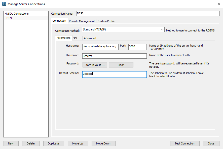
1. Click on the ‘Database' on the menu, and then click on ‘Manage Connections...'. You will see a window of ‘Manage Server Connections'.
2. Click the button ‘New' on the bottom left. Give your connection a name like ‘MySQL_WebArch'. Enter the hostname, username, password, and default schema (or database). These are on your pass card which you received at the start of the workshop. Here, the hostname is dev.spatialdatacapture.org, and the port is 3306.

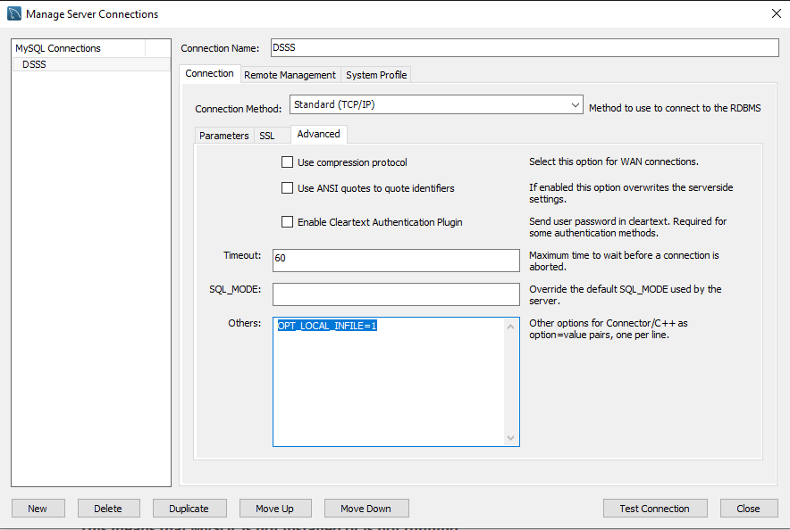
1. Change the setting of importing local files. Click the tab of ‘Advanced'. In the text box of ‘Others', enter ‘OPT_LOCAL_INFILE=1'. This enables loading a local file to the database.

1. Testing your connection and make sure it succeeds.
2. Click ‘Close' to exit. The Workbench will automatically save this connection.

Then, connect to the saved database

1. Click on the ‘Database' on the menu, and then click on ‘Connect to Database...'. You will see a window of ‘Manage Server Connections'.
2. In the new window and in the list of ‘Stored Connections', choose the one that you just created. Click ‘OK'.

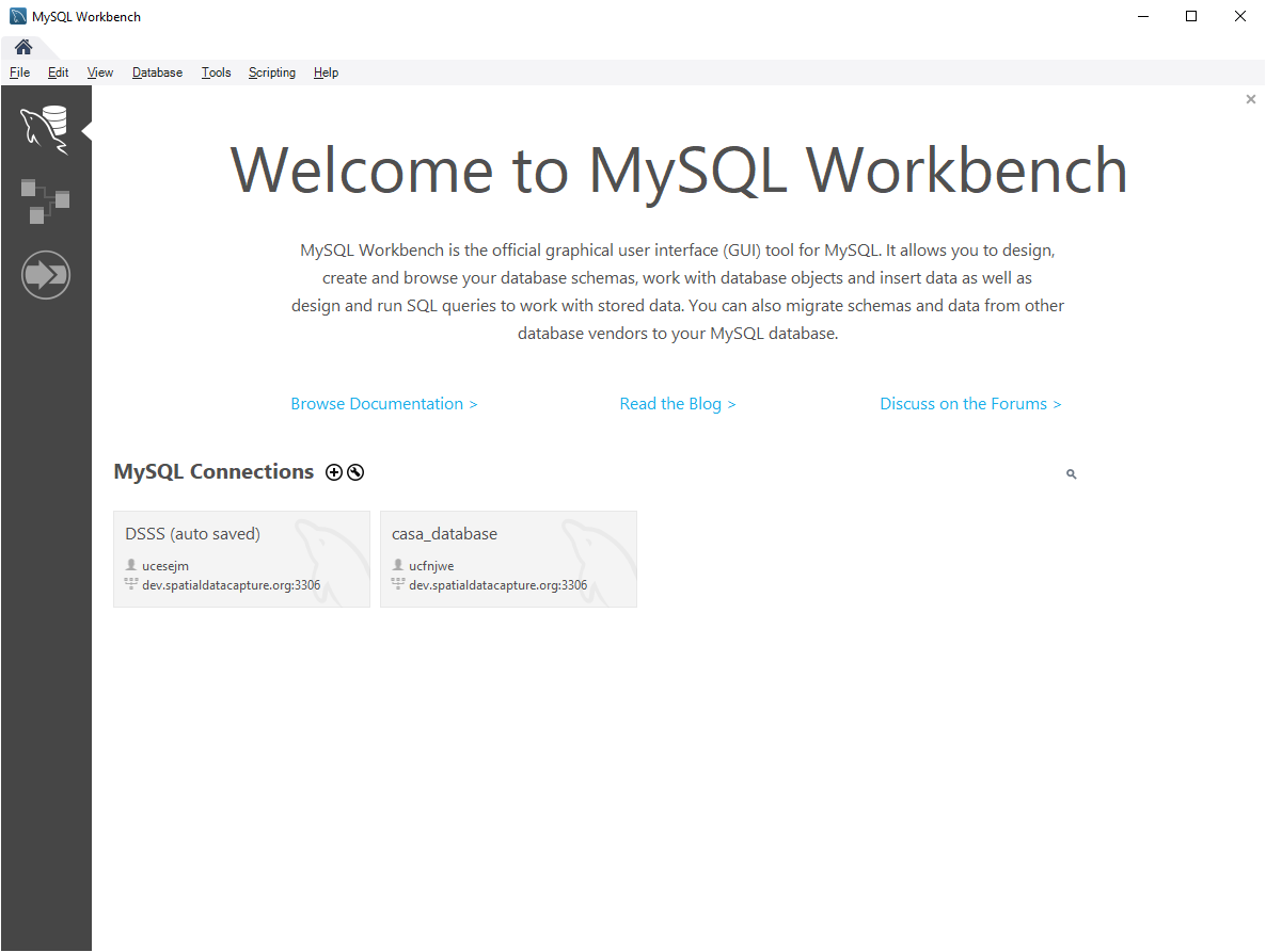
You can also use the shortcuts on the front page of MySQL workbench.

Creating your first table

A database is useless without any data stored within it. Today we'll create 3 tables that have data from photos that users have uploaded to Flickr: the photo sharing website. In this task you'll learn how to create some tables to store data within. Remember a table is a unique location to store data within, like a book sitting on a shelf of a library.
When you have connected to the database server you'll be presented with the following screen. This is the heart of the database client. Have a look around and play with the interface to make yourself familiar with the client.

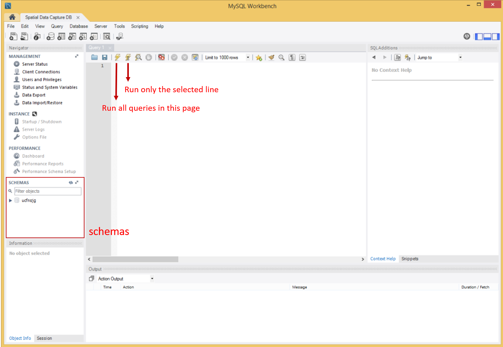
The main panel in the middle is where we enter our SQL queries to get our data from the database. The right panel shows contextual information to help us build our queries. Finally, the bottom panel is where our results appear when we execute a query on the database. There are two lightening buttons for running SQL queries, with one running all queries in the page and the other running only the selected line.
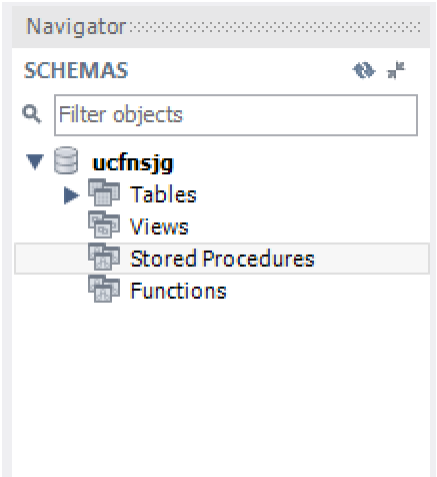
In the bottom left corner, a submenu with the title "Schemas". Schema is just a fancy name for a database. This is where your database is stored and you should be able to see you username next to the standard database symbol. Click the arrow to open up your database.

In this workbench, there are two ways to create tables: with the interface or with a query.

1. Creating a table with the interface
   1. Inside your database – right click on Tables and select Create Table
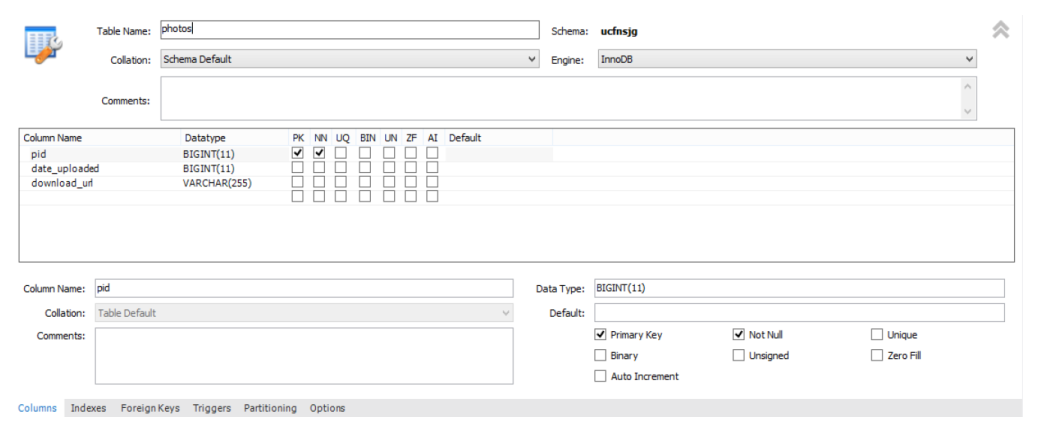
   2. Give your table a title: photos
   3. Under column name double click and enter the data for each of columns (Make sure to change the Data
      type, otherwise creating the table won't work). Here, ‘PK' and ‘NN' mean ‘Primary Key' and ‘Not Null', respectively. They are constraints to this column.
   4. Click Apply to create the table.
   
2. Creating a table with a query

When you create a table with the user interface, it's creating the following SQL query and executing it, creating the table. To create the same photos table you can enter the following query in the Query browser and click the lightening bolt (which lightening bolt should be used?).

CREATE TABLE `photo` (
	`pid` bigint(11) DEFAULT -1,
    `date_uploaded` bigint(11) DEFAULT NULL,
    `download_url` varchar(255) DEFAULT NULL
) ENGINE=InnoDB DEFAULT CHARSET=utf8;

Some tips are:

• End a SQL query with ‘;'
• There is difference between ` (called backtick or backquote) and \' (apostrophe or single quote). If you use single quotes above, it won't work. In SQL, backticks are used to indicate database, table, and column names. If you are sure that the names are not reserved or used, you can write a query without using backticks (why not try removing the backticks in the above query?). Quotes (\' or \") are used to delimit strings, and differentiate them from column names. Strings always need quotes.

Task: Can you create the following two tables with these column names and types?

Table name: metadata

Table name: photo_locations

Importing data into a table

We now have to import data into our table. Open up a browser and download the 3 data files for this workshop: http://dev.spatialdatacapture.org/data/wa_workshop_6/data.zip
Unzip the data into your user folder and make a note where the files have been created. You'll need the full path to the file in a minute.
To import the data into your table we have to run a query to read the CSV file and send it to the database for processing.

In the Query Browser enter the following command:

LOAD DATA LOCAL INFILE 'path/to/folder/flickr_2010_uk_JanFeb_photos.csv' INTO TABLE photos FIELDS TERMINATED BY ',' ENCLOSED BY '"' LINES TERMINATED BY '\n' IGNORE 1 LINES;

This command tells the database server where the file is, what table to load the data into and how the data is formatted within the CSV file. When you're ready to run the command, click the lightening bolt to execute the query.

Loading the location data

The table ‘photo_locations' contains a different type of data. The POINT data type is a special geometric type that allows the user to make spatial queries within the database. If we just tried to load the data straight from the CSV file then various errors would occur.
To fix this we need to convert the text of the POINT type data in the file and insert it in the table row by row. To do this we call LOAD DATA like this:

LOAD DATA LOCAL INFILE 'path/to/folder/FILE' INTO TABLE photo_locations FIELDS TERMINATED BY ',' ENCLOSED BY '"' LINES TERMINATED BY '\n' IGNORE 1 LINES (pid, lat, lon, @var4) SET coords = ST_GeomFromText(@var4);

Heading

Now you have all the data imported into your database we can start looking at the data.
To look at the data that you have imported into the photos table, run the following query:

SELECT * FROM photos;

This will select all the rows in the photos table. These are real photos online right now. Right click on a row to copy the URL of the photo and paste into a browser to look at the photo. Have a look around, they're over 37,000 photos in your database.
Repeat Task 3 and 4 to import the data into the other two tables and have a look around the data within the tables. Before leave you should have data in all 3 of your tables.
Hint: To retrieve all the data from the other tables, run the following commands:

SELECT * FROM photo_locations;
SELECT * FROM metadata;

Some Extra Fun

When you select all the data from photo_locations you'll see all the data contained in the table, but you'll also see that the coords column say BLOB for every value. Try viewing the data with the Spatial Viewer and see what it looks like. You may have to zoom out to see the full effect.
The reason the viewer says BLOB rather than displaying the POINT text In the data is that MySQL Workbench doesn't know how to display point data as text, as our last command forced the database to change the text into binary data via the ST_GeomFromText function!

Introduction to SQL

In this section you'll begin to use SQL (Structured Query Language) to manipulate your data. This is important stuff, and the few simple things you learn today will hold you in good stead for future database
handling.

The tutorial will introduce you to five new skills.

1. Uploading data from an SQL dump
2. Running SELECT queries
3. Extracting summary statistics and ordered lists
4. Aggregating results by shared attributes
5. Amending table contents
   Once again, we'll be working through all of this using MySQL Workbench. Just work your way through
   this worksheet; your tasks have been helpfully highlighted in a bold font.

Heading

The first thing you'll need to do is load in the new datasets that we'll be working with this section. But, rather than getting you all to create the tables and run LOAD DATA INFILE again, we're going to be nice and give
you an SQL dump of the data.

An SQL dump is a file created by a database engine to ease data transfer. It includes all of the table definitions (field names, data types, indexes etc.), and the data itself.

You can find the SQL dump file on Moodle or from here: http://casa0017.cetools.org/data/wa_workshop_6/cities.sql

Now run through the following steps to import the data:

1. Download the file (right click, Save Link As...).
2. Load up your database in MySQL Workbench 6.3 by opening the connection you setup last week
3. Open the database denoted with your username; right-click on it and select Set as Default
   Schema.
4. Go to File and Open SQL Script. Navigate to the downloaded file and open it.
   The script will open up in a new tab in Workbench. Have a look through and see if you find any familiar
   parts of the script. You'll notice too that the data is included within the file.

Run the script by pressing the Lighting Key

Then refresh your tables list (right click on Tables – Refresh) folder. You'll find two new tables – Cities
and Countries.

SELECT Queries

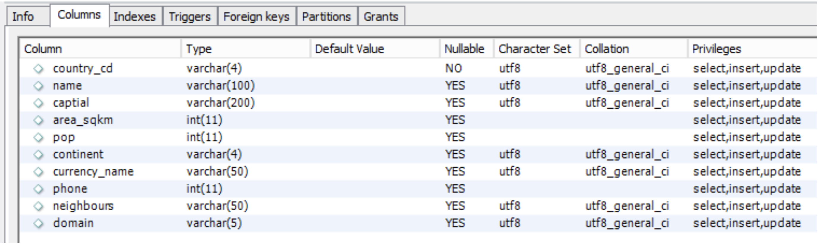
During this tutorial, we'll be working with the Countries table. Open up the table data (Right Click – Select Rows) and have a look at the data. What columns are within the dataset?

You should also check out the table definitions and see how the columns are defined. These are found through Right Click – going to Table Inspector – and then going to the Columns tab.

What data types can be found within the table?

Now, open a new SQL script by clicking on the icon in the top left of the window. Let's start
querying the data.
The first query is simple. All you're going to do is select all of the
data from the countries table. To do this you just enter the
following command and run it:

SELECT * FROM countries;

REMEMBER to add the semicolon, to make sure it remains separate from all other commands you write. You now have all of the data from the countries table. But maybe you only want certain columns from that table.

To limit this, replace the * with the column names that you want.

Add something like the following to the script, and run it again by highlighting it and pressing the Lightning Key.

SELECT name, area_sqkm FROM countries;

But still, this is not particularly interesting. Let's start putting SQL to the test by limiting what we get back.
We do this using by adding a WHERE command, after which we can add some conditions. Here is an
example:

SELECT name, pop FROM countries WHERE currency_name = 'Pound';

Instead, I want you to create a statement that returns the country name and population, ONLY when the country is found within Asia. Asian countries are denoted with the ‘AS' continent code, which must be contained within single speech marks.

Try writing this query, in the same way as the one above, to return all countries in Asia.How many rows are returned?

Now you're getting the hang of this, we will start adding additional conditions on the data, getting a bit more specific. Next, alter your last statement so you only select countries that are within Asia AND with a
population of above 1 million people. Remember to use the correct column names.

How many countries does this query return?

Now alter the statement again to limit your Asian countries to just those with a population of more than 1 million and less than 5 million people. Sounds a bit complicated, but remember this is just the same structures; you're simply adding extra conditions.

Finally, let's say we want to add countries from South America to this list. We do this by specifying that we want countries from Asia OR South America. So first, let's run this statement that brings all of our requests together.

SELECT * FROM countries WHERE continent = 'AS' AND pop > 1000000 AND pop < 5000000 OR continent = 'SA';

Notice anything wrong with the results?

You should find that while the Asian countries are limited to just those with
a population between 1m and 5m people, ALL of the South American countries are returned! The lesson is to be wary of the OR! Adding a statement using OR can potentially conflict your AND statements.

To get around this, we protect the other statements from the OR statement
by containing it within brackets. The continent conditions are grouped
together and executed separately from the population statements, like so:

SELECT * FROM countries WHERE (continent = 'AS' OR continent = 'SA') AND pop > 1000000 AND pop < 5000000;

Run this and see what you get. The results should be more in line with what we wanted – giving us just countries with limited populations, from Asia or South America.

Next, run a query that extracts the country codes and country names for all rows that have an area greater than 5000000 sqkm2.

How many countries do you get?

The queries so far have dealt mainly with simple condition statements. We also need to know how to
query text data. The SQL structure is the same, although the syntax is a bit more complicated.

Let's first try searching for a country by specific name. We did this earlier when we searched for countries from specific continents. Write a new query to extract all columns for Brazil.

However, we're often not interested in all of the text within a specific field, just some of it. SQL provides a function for searching for parts of strings within a text field. To do so we combine SQL's LIKE function with the % placeholder, to search for a part of a string. The search string can include spaces, the % takes the place of any additional text. Here is an example, try running it.

SELECT * FROM countries WHERE name LIKE '%land%';

This extracts data for all countries whose name includes the string ‘land'.

Using this same method, we can turn out attention to the neighbours
column. This field contains all of the country codes (country_cd) of all
neighbouring countries as a string.

Your final task for this section is to first, find the country code for
Russia; and then, write a query to produce all of the rows for only
the countries neighbouring Russia. Hint: You'll use Russia's country
code as the partial search string like above.

Heading

Using built-in functions, you can quickly and easily generate summary statistics using SQL. These are useful for getting a grip on the data you have, which will often run into thousands or millions of rows.

One of the first things you'll need to know about a new dataset is its row count. You can achieve this by using the COUNT(*) function. You place this where you previously requested column names, like so:

SELECT COUNT(*) FROM countries;

More importantly, it allows you to pull out row counts for queried data. Use the code above, and what you've learnt already, to find out how many countries there are in Europe only.

Other functions focus solely on extracting statistics relating to specific columns. Examples include
AVG(column), SUM(column), MAX(column) and MIN(column). In each case you replace column with the column name you are interested in. So to find out the average country population you'd run the following:

SELECT AVG(pop) FROM countries;

Likewise, SUM(pop) would give you the sum population, MAX(pop) would yield the maximum population size, and MIN(pop) would give you the minimum country population.

Try finding out the mean population size for countries in Europe alone.

Column arithmetic is another useful feature of SQL. This allows you to add, divide or multiply columns together to derive new data.

For this example, we'll calculate country population density from the fields
given. So we divide our population field by our country area field. We
provide the result with an alias using the AS function. And we add in the
country name field to make sure we know which density result relates to
which country.

The resulting command looks like this. Run it.

SELECT name, pop/area_sqkm AS population_density FROM countries;

At this point, if I were to ask you which country has the highest population density would you be able tell
me?

Yes, well maybe you already knew it was Monaco, or maybe you searched through already. But don't you want to make your life easier? Of course you do. So this takes us nicely onto ORDER BY, a very simple but very useful command. You add ORDER BY to the end of any SQL query to order the way in which the results are returned.

Again, this is a very useful function when dealing with thousands of rows of data. We can order according to any column within the given SQL command. So to order countries by area, we'd use our ORDER BY command followed by the area column name, like so. Give it a try.

SELECT * FROM countries ORDER BY area_sqkm

Now the results are all nicely ordered. But wait, I hear you think, what if I want them in the results ordered from top to bottom? Well, I have just the command you. Just add ASC or DESC after the column name, to sort in ascending or descending order.

So to reverse the order of our area results we just need to add DESC after the ordered column name to find the world's largest country. Run the command and find out what you already knew.

ORDER BY works on strings (A to Z, or Z to A) and will sort columns by their alias name too.

Aggregating Data

Often your data will be provided in a lower granularity than what you need. Aggregating data on shared attributes helps you generate summary statistics relating to grouped data. For this SQL provides the GROUP BY function.

Let's say we want to know the total populations using each type of currency. Within the current dataset this would be hard to get at, requiring us to add up the populations of each country using each type of currency. If we GROUP BY using currency_name, we can shortcut to an answer quickly.

GROUP BY allows us to aggregate rows based on shared attributes, and then generate summary statistics relating to each group. In the same way as above we select our summary functions, but then use GROUP BY to choose the column to group rows by. The GROUP BY function comes at the end of our statement, just like the ORDER BY function.

For identifying sum populations for each currency we'd run the following. Give this a try yourself.

SELECT currency_name, SUM(pop) FROM countries GROUP BY currency_name;

How many unique currencies are there? And which one is used by the most people?

Now, a task for you – use this same structure to group by continent, find the average population for each continent, and then, finally, order by average population in descending order. Which continent has the highest average population?

The End

Well done! If you've completed all the tasks above then you're finished. Go and enjoy the rest of your day! You should now have a better understanding of databases and how they work. Next week you'll learn more about SQL and how to use powerful queries to interrogate the data further.
See you all next week.